R Code Snippets
Download Code
Data Understanding in R
Histograms
Book reference: Chapter 4.3.1, page 40Histograms are generated by the function hist. The simplest way to create a histogram is to just use the corresponding attribute as an argument of the function hist, and R will automatically determine the number of bins for the histogram based on Sturge’s rule. In order to generate the histogram for the petal length of the Iris data set, the following command is sufficient:
hist(iris$Petal.Length)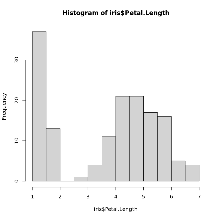
The partition into bins can also be specified directly. One of the parameters of hist is breaks. If the bins should cover the intervals \([a_{0},a_{1}),[a_{1},a_{2}),...,[a_{k−1},a_{k}]\) , then one can simply create a vector in R containing the values \(a_{i}\) and assign it to breaks. Note that \(a_{0}\) and \(a_{k}\) should be the minimum and maximum values of the corresponding attribute. If we want the boundaries for the bins at 1.0, 3.0, 4.5, 4.0, 6.1, then we would use
hist(iris$Petal.Length,breaks=c(1.0,3.0,4.5,4.0,6.9))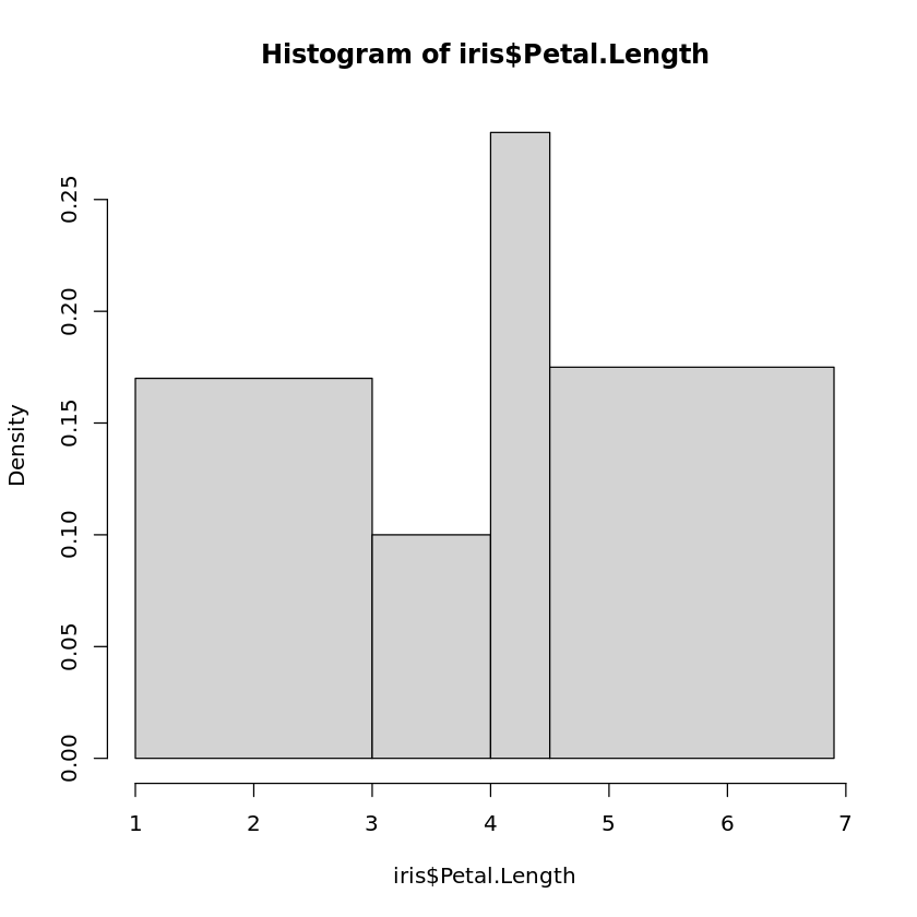
to generate the histogram. Note that in the case of bins with different length, the heights of the boxes in the histogram do not show the relative frequencies. The areas of the boxes are chosen in such a way that they are proportional to the relative frequencies.
Boxplots
Book reference: Chapter 4.3.1, page 43A boxplot for a single attribute is generated by
boxplot(iris$Petal.Length)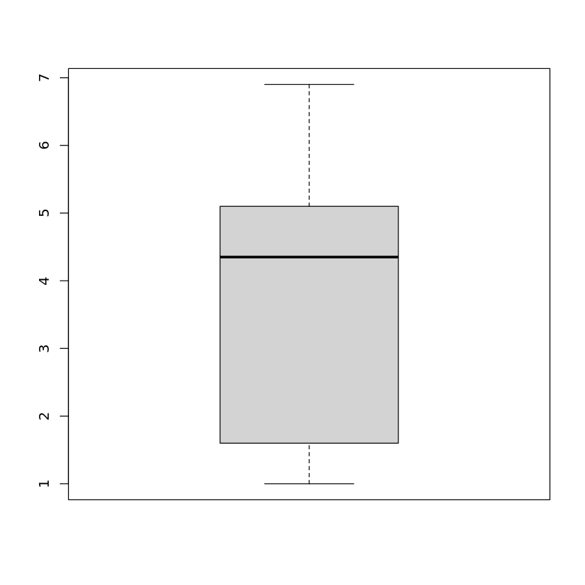
yielding the boxplot for the petal length of the Iris data set. Instead of a single attribute, we can hand over more than one attribute
boxplot(iris$Petal.Length,iris$Petal.Width)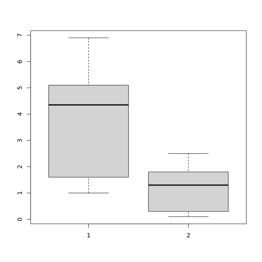
to show the boxplots in the same plot. We can even use the whole data set as an argument to see the boxplots of all attributes in one plot:
boxplot(iris)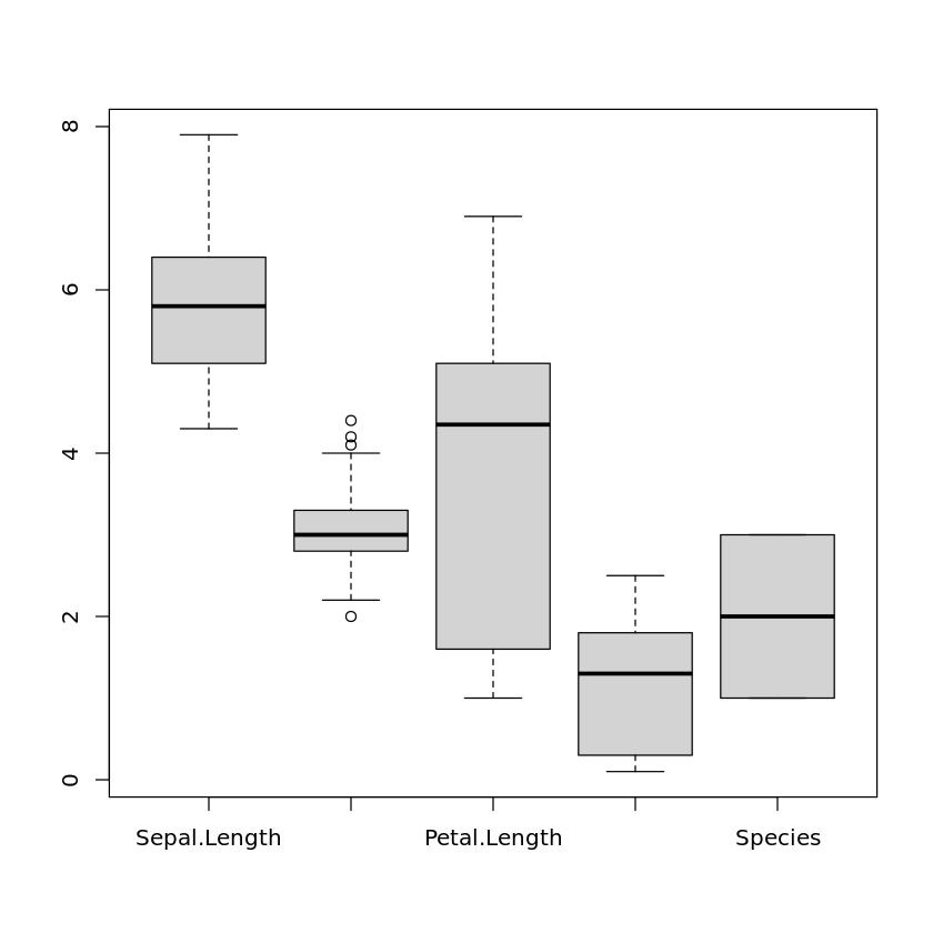
In this case, categorical attributes will be turned into numerical attributes by coding the values of the categorical attribute as 1, 2, . . . , so that these boxplots are also shown but do not really make sense.
In order to include the notches in the boxplots, we need to set the parameter notch to true:
boxplot(iris,notch=TRUE)
If one is interested in the precise values of the boxplot like the median, etc., one can use the print-command:
print(boxplot(iris$Sepal.Width))$stats
[,1]
[1,] 2.2
[2,] 2.8
[3,] 3.0
[4,] 3.3
[5,] 4.0
$n
[1] 150
$conf
[,1]
[1,] 2.935497
[2,] 3.064503
$out
[1] 4.4 4.1 4.2 2.0
$group
[1] 1 1 1 1
$names
[1] "1"
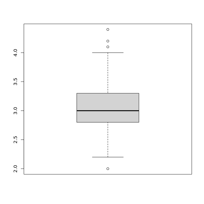
The first five values are the minimum, the first quartile, the median, the third quartile, and the maximum value of the attribute, respectively. \(n\) is the number of data. Then come the boundaries for the confidence interval for the notch, followed by the list of outliers. The last values group and names only make sense when more than one boxplot is included in the same plot. Then group is needed to identify to which attribute the outliers in the list of outliers belong. names just lists the names of the attributes.
Scatter Plots
Book reference: Chapter 4.3.1, page 45A scatter plot of the petal width against petal length of the Iris data is obtained by
plot(iris$Petal.Width,iris$Petal.Length)
All scatter plots of each attribute against each other in one diagram are created with
plot(iris)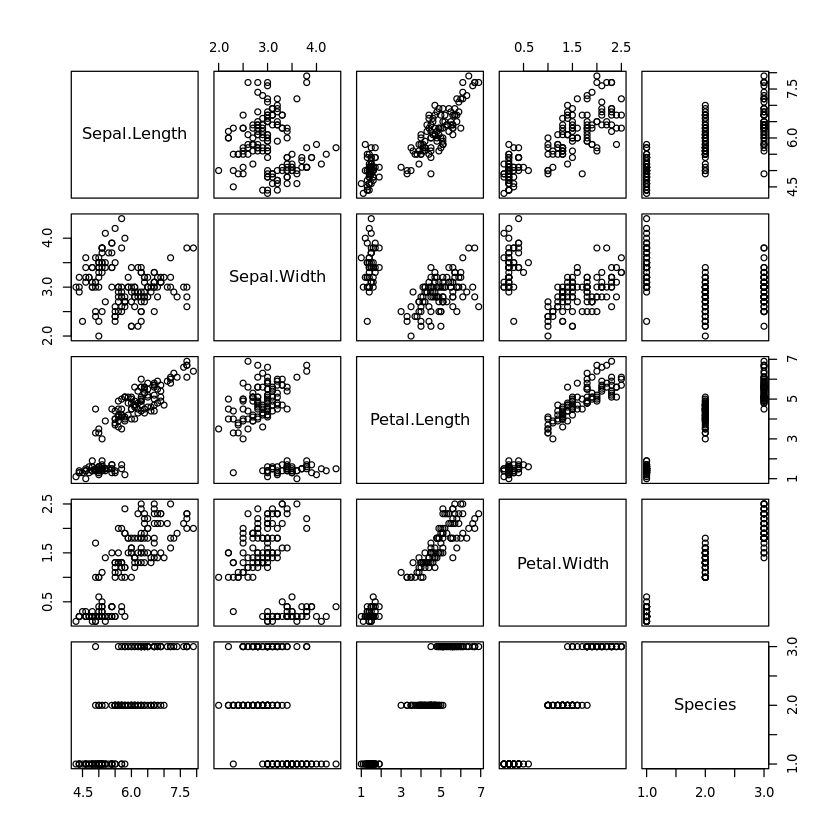
If symbols representing the values for some categorical attribute should be included in a scatter plot, this can be achieved by
plot(iris$Petal.Width,iris$Petal.Length,pch=as.numeric(iris$Species))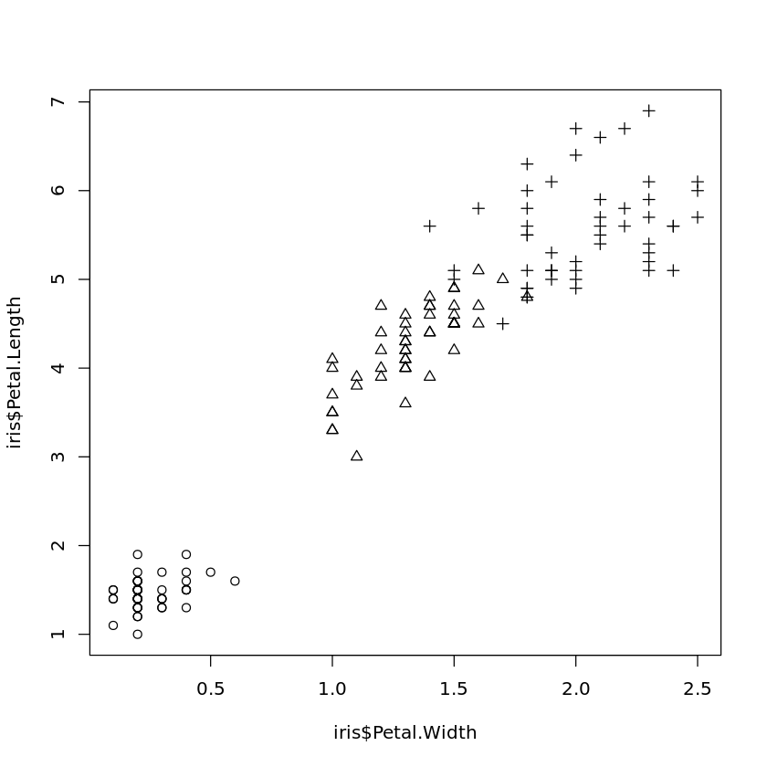
where in this example the three types of Iris are plotted with different symbols.
If there are some interesting or suspicious points in a scatter plot and one wants to find out which data records these are, one can do this by
plot(iris$Petal.Width,iris$Petal.Length)
identify(iris$Petal.Width,iris$Petal.Length)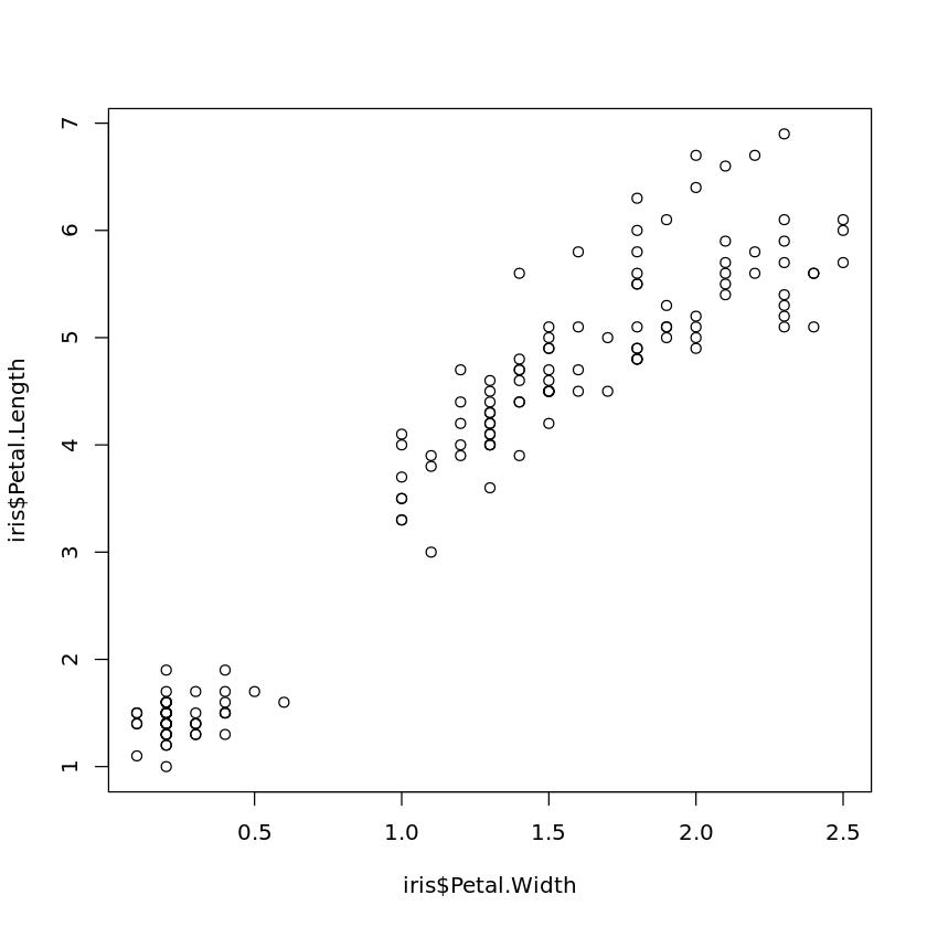
and then clicking on the points. The index of the corresponding records will be added to the scatter plot. To finish selecting points, press the ESCAPE-key.
Jitter can be added to a scatter plot in the following way:
plot(jitter(iris$Petal.Width),jitter(iris$Petal.Length))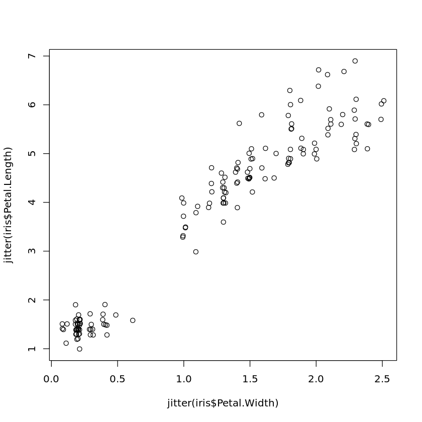
Intensity plots and density plots with hexagonal binning, as they are shown Fig. 4.9, can be generated by
plot(iris$Petal.Width,iris$Petal.Length,
     col=rgb(0,0,0,50,maxColorValue=255),pch=16)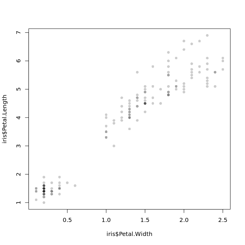
and
library(hexbin)
bin<-hexbin(iris$Petal.Width,iris$Petal.Length,xbins=50)
plot(bin)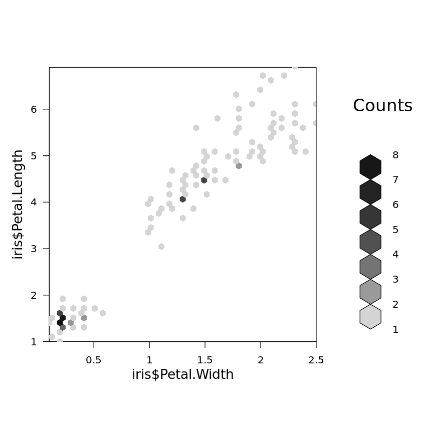
respectively, where the library hexbin does not come along with the standard version of R and needs to be installed as described in the appendix on R. Note that such plots are not very useful for such a small data sets like the Iris data set.
For three-dimensional scatter plots, the library scatterplots3d is needed and has to be installed first:
library(scatterplot3d)
scatterplot3d(iris$Sepal.Length,iris$Sepal.Width,iris$Petal.Length)
Principal Component Analysis
Book reference: Chapter 4.3.2.1, page 48PCA can be carried out with R in the following way:
species <- which(colnames(iris)=="Species")
iris.pca <- prcomp(iris[,-species],center=T,scale=T)
print(iris.pca)
Standard deviations (1, .., p=4):
[1] 1.7083611 0.9560494 0.3830886 0.1439265
Rotation (n x k) = (4 x 4):
PC1 PC2 PC3 PC4
Sepal.Length 0.5210659 -0.37741762 0.7195664 0.2612863
Sepal.Width -0.2693474 -0.92329566 -0.2443818 -0.1235096
Petal.Length 0.5804131 -0.02449161 -0.1421264 -0.8014492
Petal.Width 0.5648565 -0.06694199 -0.6342727 0.5235971
summary(iris.pca)Importance of components:
PC1 PC2 PC3 PC4
Standard deviation 1.7084 0.9560 0.38309 0.14393
Proportion of Variance 0.7296 0.2285 0.03669 0.00518
Cumulative Proportion 0.7296 0.9581 0.99482 1.00000
plot(predict(iris.pca))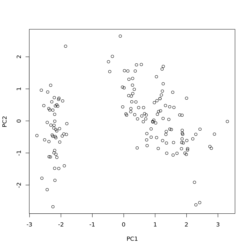
For the Iris data set, it is necessary to exclude the categorical attribute Species from PCA. This is achieved by the first line of the code and calling prcomp with iris[,-species] instead of iris.
The parameter settings center=T, scale=T, where T is just a short form of TRUE, mean that z-score standardization is carried out for each attribute before applying PCA.
The function predict can be applied in the above-described way to obtain the transformed data from which the PCA was computed. If the computed PCA transformation should be applied to another data set x, this can be achieved by
predict(iris.pca,newdata=x)where x must have the same number of columns as the data set from which the PCA has been computed. In this case, x must have four columns which must be numerical. predict will compute the full transformation, so that the above command will also yield transformed data with four columns.
Multidimensional Scaling
Book reference: Chapter 4.3.2.3, page 53MDS requires the library MASS which is not included in the standard version of R and needs installing. First, a distance matrix is needed for MDS. Identical objects leading to zero distances are not admitted. Therefore, if there are identical objects in a data set, all copies of the same object except one must be removed. In the Iris data set, there is only one pair of identical objects, so that one of them needs to be removed. The Species is not a numerical attribute and will be ignored for the distance.
library(MASS)
x <- iris[-102,]
species <- which(colnames(x)=="Species")
x.dist <- dist(x[,-species])
x.sammon <- sammon(x.dist,k=2)
plot(x.sammon$points)
Initial stress        : 0.00678
stress after  10 iters: 0.00404, magic = 0.500
stress after  12 iters: 0.00402
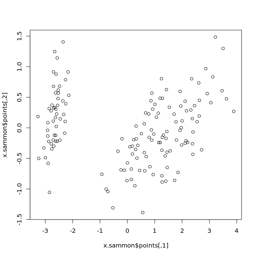
k = 2 means that MDS should reduce the original data set to two dimensions.
Note that in the above example code no normalization or z-score standardization is carried out.
Parallel Coordinates, Radar, and Star Plots
Book reference: Chapter 4.3.2.6-7, page 59Parallel coordinates need the library MASS. All attributes must be numerical. If the attribute Species should be included in the parallel coordinates, one can achieve this in the following way:
library(MASS)
x <- iris
x$Species <- as.numeric(iris$Species)
parcoord(x)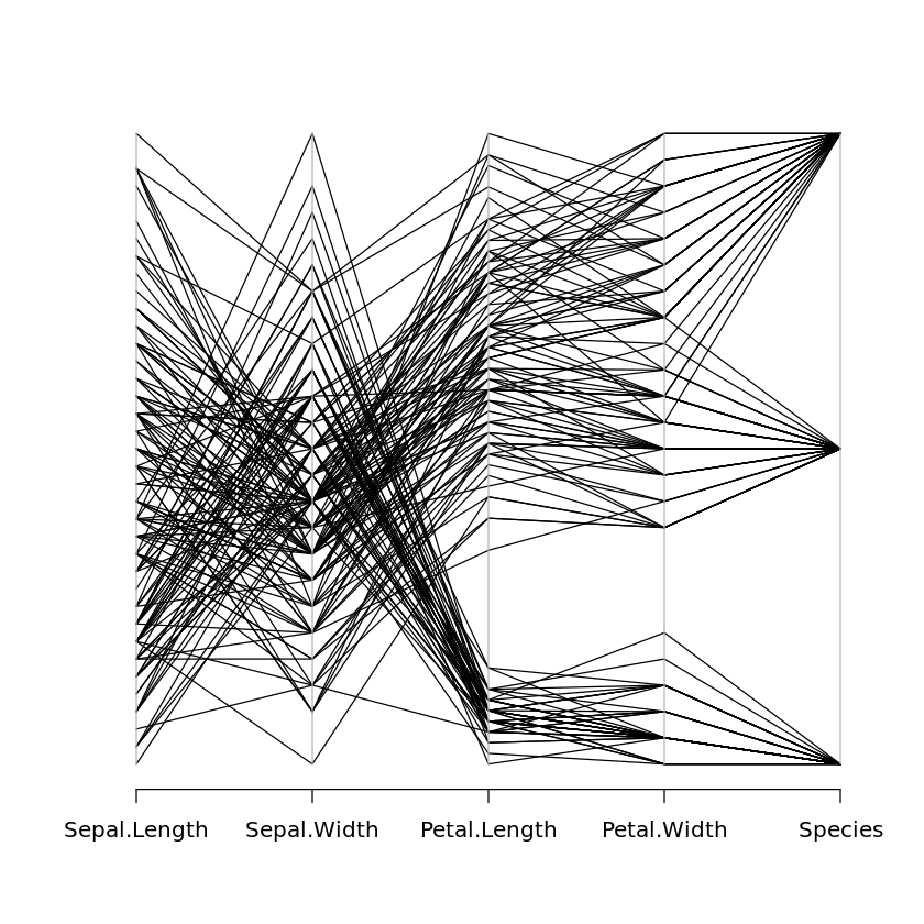
Star and radar plots are obtained by the following two commands:
stars(iris)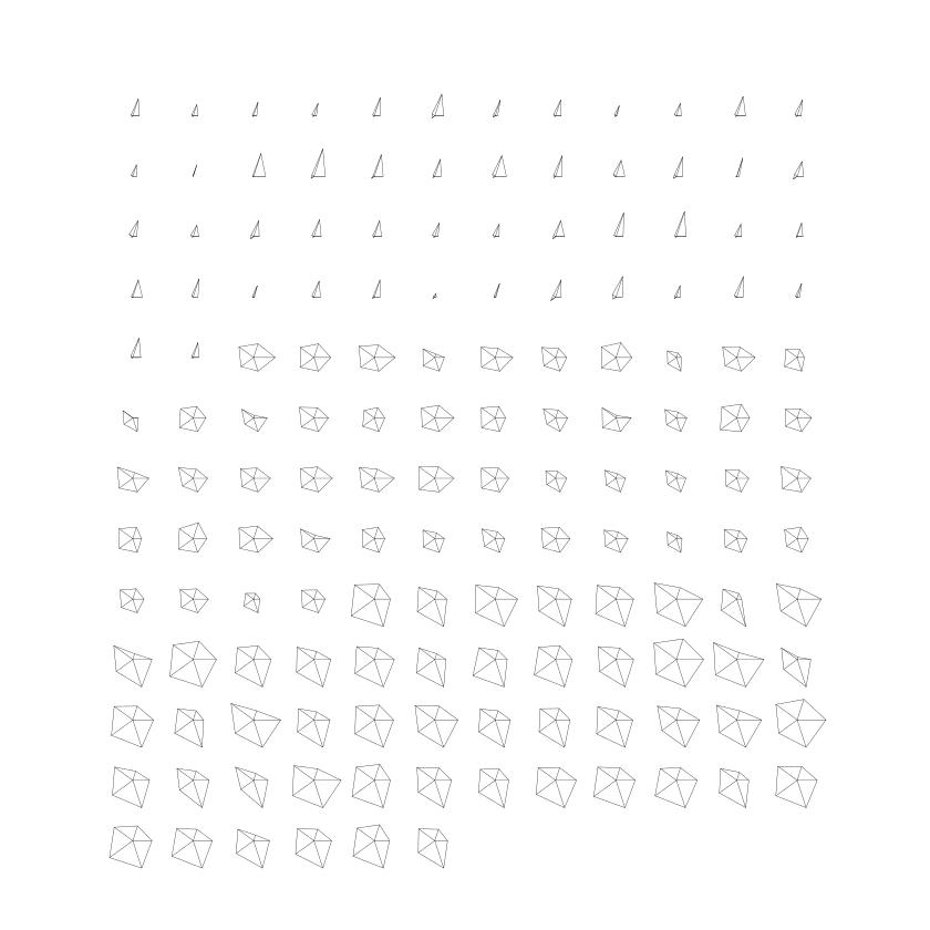
stars(iris,locations=c(0,0))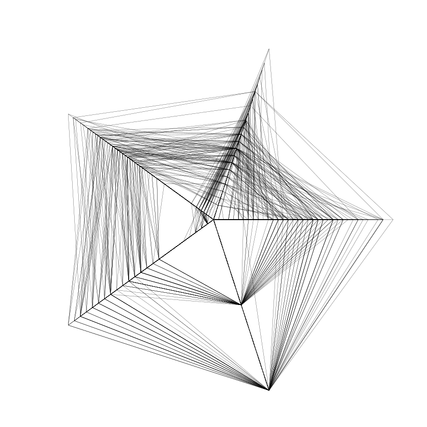
Correlation Coefficients
Book reference: Chapter 4.4, page 62Pearson’s, Spearman’s, and Kendall’s correlation coefficients are obtained by the following three commands:
cor(iris$Sepal.Length,iris$Sepal.Width)
cor.test(iris$Sepal.Length,iris$Sepal.Width,method="spearman")
cor.test(iris$Sepal.Length,iris$Sepal.Width,method="kendall")
Grubbs Test for Outlier Detection
Book reference: Chapter 4.5, page 65Grubbs test for outlier detection needs the installation of the library outliers:
library(outliers)
grubbs.test(iris$Petal.Width)
Grubbs test for one outlier data: iris$Petal.Width G = 1.70638, U = 0.98033, p-value = 1 alternative hypothesis: highest value 2.5 is an outlier
Errors and Validation in R
Book reference: Chapter 5.5.1, page 112Training and Testing Data
In order to apply the idea of using separate parts of a data set for training and testing, one needs to select random subsets of the data set. As a very simple example, we consider the Iris data set that we want to split into training and test sets. The size of the training set should contain 2/3 of the original data, and the test set 1/3. It would not be a good idea to take the first 100 records in the Iris data set for training purposes and the remaining 50 as a test set, since the records in the Iris data set are ordered with respect to the species.With such a split, all examples of Iris setosa and Iris versicolor would end up in the training set, but none of Iris versicolor, which would form the test set. Therefore, we need random sample from the Iris data set. If the records in the Iris data set were not systematically orderer, but in a random order, we could just take the first 100 records for training purposes and the remaining 50 as a test set.
Sampling and orderings in R provide a simple way to shuffle a data set, i.e., to generate a random order of the records.
First, we need to know the number n of records in our data set. Then we generate a permutation of the numbers 1, . . . , n by sampling from the vector containing the numbers 1, . . . , n, generated by the R-command c(1:n). We sample n numbers without replacement from this vector:
n <- length(iris$Species)
permut <- sample(c(1:n),n,replace=F)
Then we define this permutation as an ordering in which the records of our data set should be ordered and store the shuffled data set in the object iris.shuffled:
ord <- order(permut)
iris.shuffled <- iris[ord,]
Now define how large the fraction for the training set should be—here 2/3—and take the first two thirds of the data set as a training set and the last third as a test set:
prop.train <- 2/3  # training data consists of 2/3 of observations
k <- round(prop.train*n)
iris.training <- iris.shuffled[1:k,]
iris.test <- iris.shuffled[(k+1):n,]
The R-command sample can also be used to generate bootstrap samples by setting the parameter replace to TRUE instead of F (FALSE).
Data Preparation in R
Missing Values
Book reference: Chapter 6.2.2, page 137The logical constant NA (not available) is used to represent missing values in R. There are various methods in R that can handle missing values directly.
As a very simple example, we consider the mean value.We create a data set with one attribute with four missing values and try to compute the mean:
x <- c(3,2,NA,4,NA,1,NA,NA,5)
mean(x)
<NA>
The mean value is in this case also a missing value, since R has no information about the missing values and how to handle them. But if we explicitly say that missing values should simply be ignored for the computation of the mean value (na.rm=T), then R returns the mean value of all nonmissing values:
mean(x,na.rm=T)3
Note that this computation of the mean value implicitly assumes that the values are missing completely at random (MCAR).
Normalization and Scaling
Book reference: Chapter 6.6.3, page 153Normalization and standardization of numeric attributes can be achieved in the following way. The function is.factor returns true if the corresponding attribute is categorical (or ordinal), so that we can ensure with this function that normalization is only applied to all numerical attributes, but not to the categorical ones. With the following R-code, z-score standardization is applied to all numerical attributes:
iris.norm <- iris

# for loop over each coloumn
for (i in c(1:length(iris.norm))){
    if (!is.factor(iris.norm[,i])){
        attr.mean <- mean(iris.norm[,i])
        attr.sd <- sd(iris.norm[,i])
        iris.norm[,i] <- (iris.norm[,i]-attr.mean)/attr.sd
    }
}
Other normalization and standardization techniques can carried out in a similar manner. Of course, instead of the functions mean (for the mean value) and sd (for the standard deviation), other functions like min (for the minimum), max (for the maximum), median (for the median), or IQR (for the interquartile range) have to be used.
Finding Patterns in R
Hierarchical Clustering
Book reference: Chapter 7.1, page 159As an example, we apply hierarchical clustering to the Iris data set, ignoring the categorical attribute Species. We use the normalized Iris data set iris.norm that is constructed in Sect. 6.6.2.3. We can apply hierarchical clustering after removing the categorical attribute and can plot the dendrogram afterwards:
#
# NORMALIZATION
#

# using the iris data as an example
iris.norm <- iris

# for loop over each coloumn
for (i in c(1:length(iris.norm))){
	if (!is.factor(iris.norm[,i])){
		attr.mean <- mean(iris.norm[,i])
		attr.sd <- sd(iris.norm[,i])
		iris.norm[,i] <- (iris.norm[,i]-attr.mean)/attr.sd
	}
}
iris.num <- iris.norm[1:4]
iris.cl <- hclust(dist(iris.num), method="ward.D")
plot(iris.cl)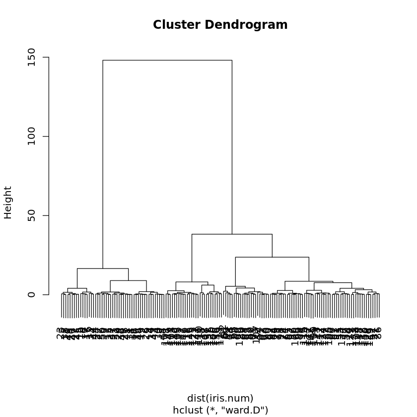
Here, the Ward method for the cluster distance aggregation function as described in Table 7.3 was chosen. For the other cluster distance aggregation functions in the table, one simply has to replace ward.D by single (for single linkage), by complete (for complete linkage), by average (for average linkage), or by centroid.
For heatmaps, the library gplots is required that needs installing first:
library(gplots)
rowv <- as.dendrogram(hclust(dist(iris.num), method="ward.D"))
colv <- as.dendrogram(hclust(dist(t(iris.num)), method="ward.D"))
heatmap.2(as.matrix(iris.num), Rowv=rowv,Colv=colv, trace="none")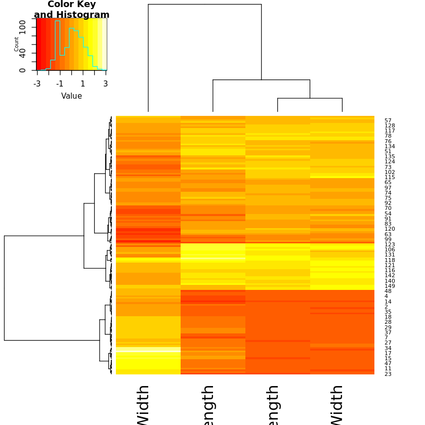
Prototype-Based Clustering
Book reference: Chapter 7.3, page 173The R-function kmeans carries out k-means clustering.
iris.km <- kmeans(iris.num,centers=3)The desired numbers of clusters is specified by the parameter centers. The location of the cluster centers and the assignment of the data to the clusters is obtained by the print function:
print(iris.km)K-means clustering with 3 clusters of sizes 50, 53, 47 Cluster means: Sepal.Length Sepal.Width Petal.Length Petal.Width 1 -1.01119138 0.85041372 -1.3006301 -1.2507035 2 -0.05005221 -0.88042696 0.3465767 0.2805873 3 1.13217737 0.08812645 0.9928284 1.0141287 Clustering vector: [1] 1 1 1 1 1 1 1 1 1 1 1 1 1 1 1 1 1 1 1 1 1 1 1 1 1 1 1 1 1 1 1 1 1 1 1 1 1 [38] 1 1 1 1 1 1 1 1 1 1 1 1 1 3 3 3 2 2 2 3 2 2 2 2 2 2 2 2 3 2 2 2 2 3 2 2 2 [75] 2 3 3 3 2 2 2 2 2 2 2 3 3 2 2 2 2 2 2 2 2 2 2 2 2 2 3 2 3 3 3 3 2 3 3 3 3 [112] 3 3 2 2 3 3 3 3 2 3 2 3 2 3 3 2 3 3 3 3 3 3 2 2 3 3 3 2 3 3 3 2 3 3 3 2 3 [149] 3 2 Within cluster sum of squares by cluster: [1] 47.35062 44.08754 47.45019 (between_SS / total_SS = 76.7 %) Available components: [1] "cluster" "centers" "totss" "withinss" "tot.withinss" [6] "betweenss" "size" "iter" "ifault"
For fuzzy c-means clustering, the library cluster is required. The clustering is carried out by the method fanny similar to kmeans:
library(cluster)
iris.fcm <- fanny(iris.num,3)
iris.fcm
The last line provides the necessary information on the clustering results, especially the membership degrees to the clusters.
Gaussian mixture decomposition automatically determining the number of clusters requires the library mclust to be installed first:
library(mclust)
iris.em <- mclustBIC(iris.num[,1:4])
iris.mod <- mclustModel(iris.num[,1:4],iris.em)
summary(iris.mod)
The last line lists the assignment of the data to the clusters.
Density-based clustering with DBSCAN is implemented in the library fpc which needs installation first:
library(fpc)
iris.dbscan <- dbscan(iris.num[,1:4],1.0,showplot=T)
iris.dbscan$cluster
The last line will print out the assignment of the data to the clusters. Singletons or outliers are marked by the number zero. The second argument in dbscan (in the above example 1:0) is the parameter " for DBSCAN. showplot=T will generate a plot of the clustering result projected to the first two dimensions of the data set.
Self Organizing Maps
Book reference: Chapter 7.5, page 187The library som provides methods for self organizing maps. The library som needs to be installed:
library(som)
iris.som <- som(iris.num,xdim=5,ydim=5)
plot(iris.som)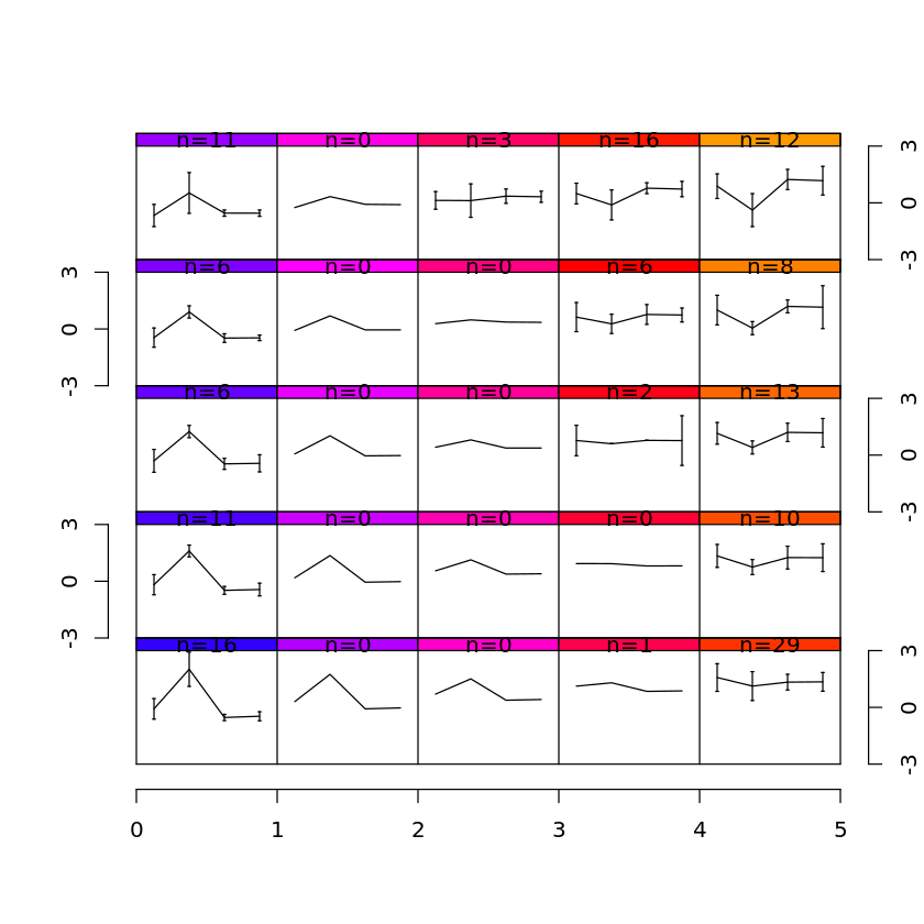
xdim and ydim define the number of nodes in the mesh in x- and y-directions, respectively. plot will show, for each node in the mesh, a representation of the values in the form of parallel coordinates.
Association Rules
Book reference: Chapter 7.9, page 189For association rule mining, the library arules is required in which the function apriori is defined. This library does not come along with R directly and needs to be installed first.
Here we use an artificial data set basket that we enter manually. The data set is a list of vectors where each vector contains the items that were bought:
library(arules)
baskets <- list(c("a","b","c"), c("a","d","e"),
                c("b","c","d"), c("a","b","c","d"),
                c("b","c"), c("a","b","d"),
                c("d","e"), c("a","b","c","d"),
                c("c","d","e"), c("a","b","c"))
rules <- apriori(baskets,parameter = list(supp=0.1,conf=0.8,target="rules"))
inspect(rules)
Loading required package: Matrix
Attaching package: ‘arules’
The following objects are masked from ‘package:base’:
abbreviate, write
Apriori

Parameter specification:
 confidence minval smax arem  aval originalSupport maxtime support minlen
        0.8    0.1    1 none FALSE            TRUE       5     0.1      1
 maxlen target  ext
     10  rules TRUE

Algorithmic control:
 filter tree heap memopt load sort verbose
    0.1 TRUE TRUE  FALSE TRUE    2    TRUE

Absolute minimum support count: 1

set item appearances ...[0 item(s)] done [0.00s].
set transactions ...[5 item(s), 10 transaction(s)] done [0.00s].
sorting and recoding items ... [5 item(s)] done [0.00s].
creating transaction tree ... done [0.00s].
checking subsets of size 1 2 3 4 done [0.00s].
writing ... [9 rule(s)] done [0.00s].
creating S4 object  ... done [0.00s].
    lhs        rhs support confidence coverage lift     count
[1] {e}     => {d} 0.3     1.0000000  0.3      1.428571 3
[2] {a}     => {b} 0.5     0.8333333  0.6      1.190476 5
[3] {b}     => {c} 0.6     0.8571429  0.7      1.224490 6
[4] {c}     => {b} 0.6     0.8571429  0.7      1.224490 6
[5] {a,e}   => {d} 0.1     1.0000000  0.1      1.428571 1
[6] {c,e}   => {d} 0.1     1.0000000  0.1      1.428571 1
[7] {a,b}   => {c} 0.4     0.8000000  0.5      1.142857 4
[8] {a,c}   => {b} 0.4     1.0000000  0.4      1.428571 4
[9] {a,c,d} => {b} 0.2     1.0000000  0.2      1.428571 2
The last command lists the rules with their support, confidence, and lift.
Finding Explanations
Decision tree
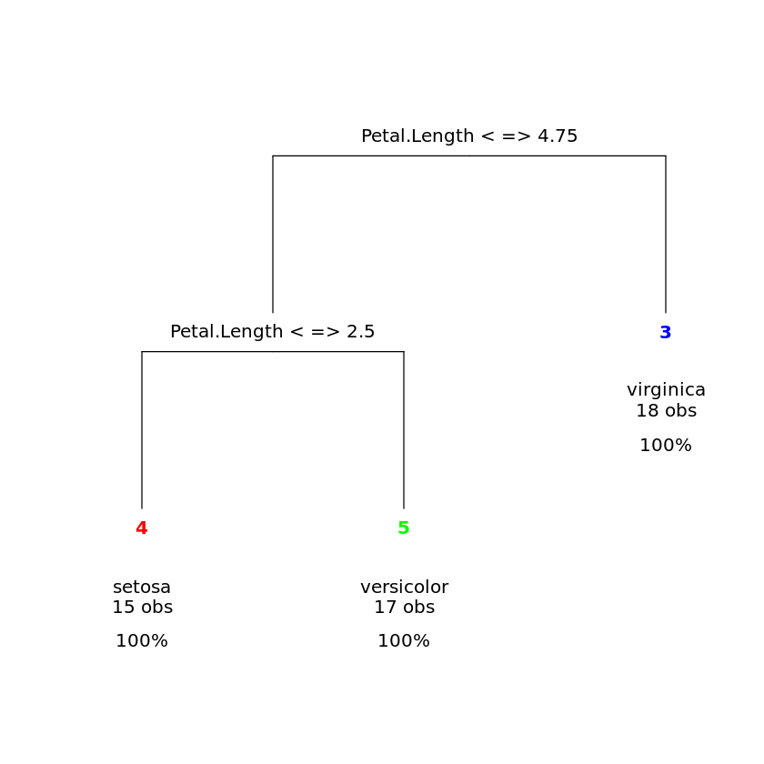
Book reference: Chapter 8.1, page 220R also allows for much finer control of the decision tree construction. The script below demonstrates how to create a simple tree for the Iris data set using a training set of 100 records. Then the tree is displayed, and a confusion matrix for the test set—the remaining 50 records of the Iris data set—is printed. The libraries rpart, which comes along with the standard installation of R, and rattle, that needs to be installed, are required:
library(rpart)
iris.train <- c(sample(1:150,50))
iris.dtree <- rpart(Species~.,data=iris,subset=iris.train)
library(rattle)
drawTreeNodes(iris.dtree)
table(predict(iris.dtree,iris[-iris.train,],type="class"),
iris[-iris.train,"Species"])Loading required package: tibble Loading required package: bitops Rattle: A free graphical interface for data science with R. Version 5.4.0 Copyright (c) 2006-2020 Togaware Pty Ltd. Type 'rattle()' to shake, rattle, and roll your data.
             setosa versicolor virginica
  setosa         35          0         0
  versicolor      0         27         1
  virginica       0          6        31
In addition to many options related to tree construction, R also offers many ways to beautify the graphical representation. We refer to R manuals for more details.
Naive Bayes Classifiers
Book reference: Chapter 8.2, page 230Naive Bayes classifiers use normal distributions by default for numerical attributes. The package e1071 must be installed first:
library(e1071)
iris.train <- c(sample(1:150,75))
iris.nbayes <- naiveBayes(Species~.,data=iris,subset=iris.train)
table(predict(iris.nbayes,iris[-iris.train,],type="class"),
      iris[-iris.train,"Species"])
setosa versicolor virginica setosa 28 0 0 versicolor 0 22 1 virginica 0 2 22
As in the example of the decision tree, the Iris data set is split into a training and a test data set, and the confusion matrix is printed. The parameters for the normal distributions of the classes can be obtained in the following way:
print(iris.nbayes)Naive Bayes Classifier for Discrete Predictors
Call:
naiveBayes.default(x = X, y = Y, laplace = laplace)
A-priori probabilities:
Y
setosa versicolor virginica
0.2933333 0.3466667 0.3600000
Conditional probabilities:
Sepal.Length
Y [,1] [,2]
setosa 4.972727 0.3781935
versicolor 6.034615 0.5059188
virginica 6.555556 0.5401804
Sepal.Width
Y [,1] [,2]
setosa 3.422727 0.4264268
versicolor 2.807692 0.2682135
virginica 2.937037 0.3236191
Petal.Length
Y [,1] [,2]
setosa 1.413636 0.1457181
versicolor 4.315385 0.4333057
virginica 5.514815 0.4888792
Petal.Width
Y [,1] [,2]
setosa 0.2409091 0.09081164
versicolor 1.3307692 0.18279875
virginica 2.0185185 0.30386869
If Laplace correction should be applied for categorical attribute, this can be achieved by setting the parameter laplace to the desired value when calling the function naiveBayes.
Regression
Book reference: Chapter 8.3, page 241Least squares linear regression is implemented by the function lm (linear model). As an example, we construct a linear regression function to predict the petal width of the Iris data set based on the other numerical attributes:
iris.lm <- lm(iris$Petal.Width ~ iris$Sepal.Length
              + iris$Sepal.Width + iris$Petal.Length)
summary(iris.lm)
Call:
lm(formula = iris$Petal.Width ~ iris$Sepal.Length + iris$Sepal.Width +
iris$Petal.Length)
Residuals:
Min 1Q Median 3Q Max
-0.60959 -0.10134 -0.01089 0.09825 0.60685
Coefficients:
Estimate Std. Error t value Pr(>|t|)
(Intercept) -0.24031 0.17837 -1.347 0.18
iris$Sepal.Length -0.20727 0.04751 -4.363 2.41e-05 ***
iris$Sepal.Width 0.22283 0.04894 4.553 1.10e-05 ***
iris$Petal.Length 0.52408 0.02449 21.399 < 2e-16 ***
---
Signif. codes: 0 ‘***’ 0.001 ‘**’ 0.01 ‘*’ 0.05 ‘.’ 0.1 ‘ ’ 1
Residual standard error: 0.192 on 146 degrees of freedom
Multiple R-squared: 0.9379, Adjusted R-squared: 0.9366
F-statistic: 734.4 on 3 and 146 DF, p-value: < 2.2e-16
The summary provides the necessary information about the regression result, including the coefficient of the regression function.
If we want to use a polynomial as the regression function, we need to protect the evaluation of the corresponding power by the function I inhibiting interpretation. As an example, we compute a regression function to predict the petal width based on a quadratic function in the petal length:
iris.lm <- lm(iris$Petal.Width ~ iris$Petal.Length +
              I(iris$Petal.Length^2))
summary(iris.lm)
Call:
lm(formula = iris$Petal.Width ~ iris$Petal.Length + I(iris$Petal.Length^2))
Residuals:
Min 1Q Median 3Q Max
-0.56213 -0.12392 -0.01555 0.13547 0.64105
Coefficients:
Estimate Std. Error t value Pr(>|t|)
(Intercept) -0.386781 0.079883 -4.842 3.22e-06 ***
iris$Petal.Length 0.433833 0.053652 8.086 2.10e-13 ***
I(iris$Petal.Length^2) -0.002569 0.007501 -0.342 0.732
---
Signif. codes: 0 ‘***’ 0.001 ‘**’ 0.01 ‘*’ 0.05 ‘.’ 0.1 ‘ ’ 1
Residual standard error: 0.2071 on 147 degrees of freedom
Multiple R-squared: 0.9272, Adjusted R-squared: 0.9262
F-statistic: 935.7 on 2 and 147 DF, p-value: < 2.2e-16
Robust regression requires the library MASS, which needs installation. Otherwise it is handled in the same way as least squares regression, using the function rlm instead of lm:
library(MASS)
iris.rlm <- rlm(iris$Petal.Width ~ iris$Sepal.Length
                + iris$Sepal.Width + iris$Petal.Length)
summary(iris.rlm)
Call: rlm(formula = iris$Petal.Width ~ iris$Sepal.Length + iris$Sepal.Width +
iris$Petal.Length)
Residuals:
Min 1Q Median 3Q Max
-0.606532 -0.099003 -0.009158 0.101636 0.609940
Coefficients:
Value Std. Error t value
(Intercept) -0.2375 0.1771 -1.3412
iris$Sepal.Length -0.2062 0.0472 -4.3713
iris$Sepal.Width 0.2201 0.0486 4.5297
iris$Petal.Length 0.5231 0.0243 21.5126
Residual standard error: 0.1492 on 146 degrees of freedom
The default method is based on Huber’s error function. If Tukey’s biweight should be used, the parameter method should be changed in the following way:
# ridge regression with Tukey's biweight
iris.rlm <- rlm(iris$Petal.Width ~ iris$Sepal.Length
                + iris$Sepal.Width + iris$Petal.Length,
                method="MM")
summary(iris.rlm)
Call: rlm(formula = iris$Petal.Width ~ iris$Sepal.Length + iris$Sepal.Width +
iris$Petal.Length, method = "MM")
Residuals:
Min 1Q Median 3Q Max
-0.60608 -0.09975 -0.01030 0.10375 0.61963
Coefficients:
Value Std. Error t value
(Intercept) -0.1896 0.1718 -1.1036
iris$Sepal.Length -0.2152 0.0457 -4.7036
iris$Sepal.Width 0.2181 0.0471 4.6276
iris$Petal.Length 0.5252 0.0236 22.2689
Residual standard error: 0.1672 on 146 degrees of freedom
A plot of the computed weights can be obtained by the following command:
plot(iris.rlm$w)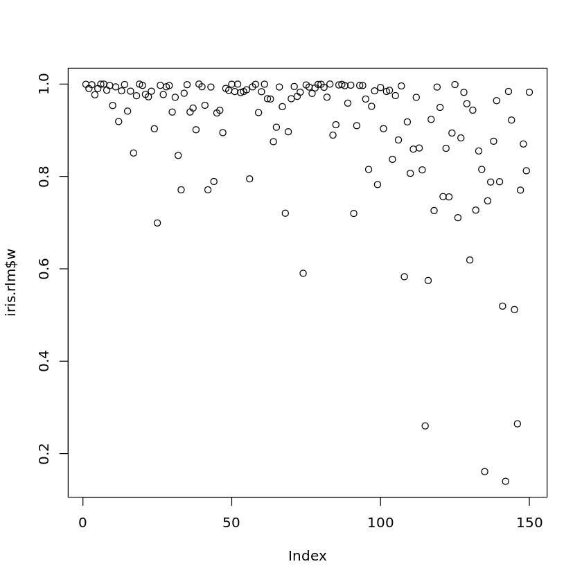
Predictors
Nearest Neighbor Classifiers
Book reference: Chapter 9.1, page 275A nearest-neighbor classifier based on the Euclidean distance is implemented in the package class in R. To show how to use the nearest-neighbor classifier in R, we use splitting of the Iris data set into a training set iris.training and test set iris.test as it was demonstrated in Sect. 5.6.2. The function knn requires a training and a set with only numerical attributes and a vector containing the classifications for the training set. The parameter k determines how many nearest neighbors are considered for the classification decision.
# generating indices for shuffling
n <- length(iris$Species)
permut <- sample(c(1:n),n,replace=F)

# shuffling the observations
ord <- order(permut)
iris.shuffled <- iris[ord,]

# splitting into training and testing data
prop.train <- 2/3  # training data consists of 2/3 of observations
k <- round(prop.train*n)
iris.training <- iris.shuffled[1:k,]
iris.test <- iris.shuffled[(k+1):n,]
library(class)
iris.knn <- knn(iris.training[,1:4],iris.test[,1:4],iris.training[,5],k=3)
table(iris.knn,iris.test[,5])iris.knn setosa versicolor virginica setosa 18 0 0 versicolor 0 18 0 virginica 0 1 13
The last line prints the confusion matrix.
Neural Networks
Book reference: Chapter 9.2, page 282For the example of multilayer perceptrons in R, we use the same training and test data as for the nearest-neighbor classifier above. The multilayer perceptron can only process numerical values. Therefore, we first have to transform the categorical attribute Species into a numerical attribute:
x <- iris.training
x$Species <- as.numeric(x$Species)
The multilayer perceptron is constructed and trained in the following way, where the library neuralnet needs to be installed first:
library(neuralnet)
iris.nn <- neuralnet(Species + Sepal.Length ~
                     Sepal.Width + Petal.Length + Petal.Width, x,
                     hidden=c(3))
The first argument of neuralnet defines that the attributes Species and sepal length correspond to the output neurons. The other three attributes correspond to the input neurons. x specifies the training data set. The parameter hidden defines how many hidden layers the multilayer perceptron should have and how many neurons in each hidden layer should be. In the above example, there is only one hidden layer with three neurons. When we replace c(3) by c(4,2), there would be two hidden layers, one with four and one with two neurons.
The training of the multilayer perceptron can take some time, especially for larger data sets.
When the training is finished, the multilayer perceptron can be visualized:
plot(iris.nn)The visualization includes also dummy neurons as shown in Fig. 9.4.
The output of the multilayer perceptron for the test set can be calculated in the following way. Note that we first have to remove the output attributes from the test set:
y <- iris.test
y <- y[-5]
y <- y[-1]
y.out <- compute(iris.nn,y)
We can then compare the target outputs for the training set with the outputs from the multilayer perceptron. If we want to compute the squared errors for the second output neuron -— the sepal length —- we can do this in the following way:
y.sqerr <- (y[1] - y.out$net.result[,2])^2Support Vector Machines
Book reference: Chapter 9.4, page 297For support vector machine, we use the same training and test data as already for the nearest-neighbor classifier and for the neural networks. A support vector machine to predict the species in the Iris data set based on the other attributes can be constructed in the following way. The package e1071 is needed and should be installed first if it has not been installed before:
library(e1071)
iris.svm <- svm(Species ~ ., data = iris.training)
table(predict(iris.svm,iris.test[1:4]),iris.test[,5])
setosa versicolor virginica setosa 18 0 0 versicolor 0 19 1 virginica 0 0 12
The last line prints the confusion matrix for the test data set.
The function svm works also for support vector regression. We could, for instance, use
iris.svm <- svm(Petal.Width ~ ., data = iris.training)
sqerr <- (predict(iris.svm,iris.test[-4])-iris.test[4])^2
to predict the numerical attribute petal width based on the other attributes and to compute the squared errors for the test set.
Ensemble Methods
Book reference: Chapter 9.5, page 304As an example for ensemble methods, we consider random forest with the training and test data of the Iris data set as before. The package randomForest needs to be installed first:
library(randomForest)
iris.rf <- randomForest(Species ~., iris.training)
table(predict(iris.rf,iris.test[1:4]),iris.test[,5])
setosa versicolor virginica setosa 18 0 0 versicolor 0 19 1 virginica 0 0 12
In this way, a random forest is constructed to predict the species in the Iris data set based on the other attributes. The last line of the code prints the confusion matrix for the test data set.